Chapter 3 The Push-Pull Method
3.1 Introduction
Suppose we have two nonnegative matrices \(R,C^T\in\mathbb{R}^{n\times n}\) and two induced digraph \(\mathcal{G}_R, \mathcal{G}_{C^T}\). Suppose each agent \(i\in\mathcal{N}\) can actively and reliably push information out to its neighbor \(l\in\mathcal{N}^{out}_{C,i}\subset\mathcal{N}\) and pull information from its neighbor \(j\in\mathcal{N}^{in}_{R,i}\subset\mathcal{N}\). Matrix \(R=(r_{ij})\in\mathbb{R}^{n\times n}\) denotes the pulling weights that agent \(i\) pulls information from agent \(j\). Thus the row sum of \(R\) should be \(1\), i.e. \(R\boldsymbol 1 = \boldsymbol 1\) and \(r_{ij}\geq 0\). That is to say, matrix \(R\) is row-stochastic. Similarly, \(C = (c_{ij})\in\mathbb{R}^{n\times n}\) denotes the pushing weights that agent \(i\) pushes information to agent \(j\). In other words, it denotes the pulling weights that agent \(j\) pulls information from agent \(i\). Hence \(C^T\boldsymbol 1=\boldsymbol 1\), i.e. \(\boldsymbol 1^T C=\boldsymbol 1^T, c_{ji}\geq 0\). Moreover, for agent \(i\), it will have no problem getting information from itself, hence \(r_{ii}>0, c_{ii}>0\). Assumption 3.1 will gurantee this.
\
Assumption 3.2 is to say that at least one agent is connected to all other agents in this system(thus they should be both “pulled” and “pushed”), which is weaker to assume that the system is connected. Hence these agents are significant and we must assume at least one of them contribute to the update, i.e. assumption 3.3.
Figure 3.12 shows the master-workers architecture in distributed optimization, which fits the assumption 3.2 when \(\mathcal{R}_{R} \cap \mathcal{R}_{\mathbf{C}^{\top}}=\{\text{master node}\}\).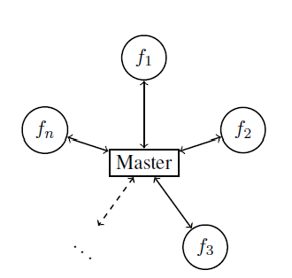
Figure 3.1: Master-Workers Architecture
Assumption 3.2 and 3.1 would lead to the following lemma 3.1,
Lemma 3.1 Under assumptions 3.1 and 3.2, the matrix \(R\) has a unique nonnegative left eigenvector \(u^T\)(w.r.t. eigenvalue 1) with \(u^T\boldsymbol1 = n\), and the matrix \(C\) has a unique nonnegative right eigenvector \(v\) (w.r.t. eigenvalue 1) with \(\boldsymbol1^T v = n\), i.e., \[ u^T R = 1\cdot u^T \]
\[ Cv = 1\cdot v \]
Moreover, \(u^T\) (resp., \(v\)) is nonzero only on the entries associated with agents \(i\in\mathcal{R}_R\)(resp., \(j\in\mathcal{R}_{C^T}\)), and \(u^Tv>0\).
The idea of Push-Pull Gradient Methods is that, at each iteration step \(k\), agent \(i\) updates its local copy of decision variable \(x_{i,k+1}\in\mathbb R^p\) according to the information it pulls from its nearby agents based on the corresponding pulling weights \((r_{i1},r_{i2},...,r_{in})\). Then it will also update the information stored in an auxiliary variable \(y_{i, k+1}\in\mathbb{R}^p\)
Algorithm3.1 (Push-Pull Method) Each agent \(i\) chooses its local step size \(\alpha_i\geq0\) and initilized with an arbitary \(x_{i,0}\in\mathbb{R}^p, y_{i,0}=\nabla f_i(x_{i,0})\).
For k = 0, 1, …,
For \(i\in\mathcal{N}\),
\(x_{i, k+1} = \sum\limits_{j=1}^nr_{ij}(x_{j, k}-\alpha_j y_{j, k})\) (Pull)
- \(y_{i, k+1} = \sum\limits_{j=1}^nc_{ij}y_{j,k}+\nabla f_i(x_{i,k+1})-\nabla f_i(x_{i,k})\)(Push)
3.2 Analysis of Convergence
we first bound \((\Vert\bar x_{k+1}-x^*\Vert_2, \Vert X_{k+1}-\boldsymbol1\bar x_{k+1}\Vert_R,\Vert Y_{k+1}-v\bar y_{k+1}\Vert_C)^T\) by a linear combination in terms of their previous values. Then based on lemma 3.2, we derive how should we choose the step sizes \(\alpha_i,i=1,2,...,n\) so that \(\rho(A)<1\).
In this chapter, we define the matrix norm of \(X\in\mathbb R^{n\times p }\) using definition 3.1.
For example, when \(\Vert\cdot\Vert\) is the \(2-\)norm, then the matrix norm under definition 3.1 is the Frobenius norm.
While in the chapter of distributed stochastic gradient tracking method, we use Frobenius norm as matrix norm.
3.2.1 Relationship between two iteration steps
We first give definition of \(\bar x_k\) and \(\bar y_k\).
\[\begin{equation} \bar x_k := \frac{1}{n}u^TX_k\in\mathbb{R}^{1\times p},\quad \bar y_k:= \frac{1}{n}\boldsymbol 1 \nabla F(X_k)\in\mathbb{R}^{1\times p} \tag{3.3} \end{equation}\]The authors do not define \(\bar x_k\) as \(\frac{1}{n}\boldsymbol 1^TX_k\) is because the pulling information is subject to the graph \(\mathcal{G}_R\), which may not be strongly connected. Thus agent \(i\) could never use information from agent \(j\not\in N^{in}_{R,i}\).
For the pull step,
\[\begin{equation} \bar x_{k+1} = \frac{1}{n}u^TX_{k+1}\stackrel{\text{pull step}}{=}\frac{1}{n}u^TR(X_k-\boldsymbol\alpha Y_k)=\bar x_k-\frac{1}{n}u^T\boldsymbol\alpha Y_k \tag{3.4} \end{equation}\]Hence,
\[\begin{align} X_{k+1}-\boldsymbol1\bar x_{k+1}&= R(X_k-\boldsymbol\alpha Y_k)-\boldsymbol1(\bar x_k-\frac{1}{n}u^T\boldsymbol\alpha Y_k)\\ &=(R-\frac{\boldsymbol 1 u^T}{n})(X_k-\boldsymbol 1\bar x_k)- (R-\frac{\boldsymbol 1 u^T}{n})\boldsymbol\alpha Y_k+\frac{\boldsymbol 1 u^T}{n}(X_k-\boldsymbol 1\bar x_k)\\ &=(R-\frac{\boldsymbol 1 u^T}{n})(X_k-\boldsymbol 1\bar x_k)- (R-\frac{\boldsymbol 1 u^T}{n})\boldsymbol\alpha Y_k \tag{3.5} \end{align}\]This is because \(\frac{\boldsymbol 1 u^T}{n}(X_k-\boldsymbol 1\bar x_k)=\bar x_k-\frac{u^T\boldsymbol1}{n}\bar x_k=0\) according to lemma 3.1.
To see what does this difference mean, we rewrite \(X_{k+1}-\boldsymbol1\bar x_{k+1}\) as
\[\begin{equation} (x_1-\frac{1}{n}\sum_{i=1}^n u_i x_i,...,x_n-\frac{1}{n}\sum_{i=1}^n u_i x_i)^T\in\mathbb{R}^{n\times p} \end{equation}\]where \(u=(u_1,...,u_n)^T\in\mathbb{R}^n,x_i\in\mathbb{R}^p\). It denotes the difference between each agent \(i\)’s decision variable and the overall weighted mean.
For the push step,
\[\begin{align} Y_{k+1}-v\bar y_{k+1}&\stackrel{\text{push step}}=CY_k+\nabla F(X_{k+1})-\\ &\nabla F(X_k)-v[\frac{1}{n}\boldsymbol1(CY_k+\nabla F(X_{k+1})-\nabla F(X_k))]\\ &=CY_k-v\bar y_k+(I-\frac{v\boldsymbol1^T}{n})(\nabla F(X_{k+1})-\nabla F(X_k))\\ &=(C-\frac{v\boldsymbol1^T}{n})(Y_k-v\bar y_k)+(I-\frac{v\boldsymbol1^T}{n})(\nabla F(X_{k+1})-\nabla F(X_k))+\\ &Cv\bar y_k+\frac{v\boldsymbol1^T}{n}Y_k-\frac{v\boldsymbol1^Tv}{n}\bar y_k-v\bar y_k\\ &=(C-\frac{v\boldsymbol1^T}{n})(Y_k-v\bar y_k)+(I-\frac{v\boldsymbol1^T}{n})(\nabla F(X_{k+1})-\nabla F(X_k)) \tag{3.6} \end{align}\]where \[ \frac{1}{n}v\boldsymbol1^TCY_k=v\bar y_k \]
\[ Cv\bar y_k+\frac{v\boldsymbol1^T}{n}Y_k-\frac{v\boldsymbol1^Tv}{n}\bar y_k-v\bar y_k=v\bar y_k+v\bar y_k-v\bar y_k-v\bar y_k=0 \] This is because the column-stochastic of \(C\), i.e. \(\mathbf{1}^TC=\mathbf{1}^T\) and lemma 3.1.
Similarly, we can rewrite \(Y_{k+1}-v\bar y_{k+1}\) as \[\begin{equation} (y_1-\frac{1}{n}v_1\sum_{i=1}^ny_i,...,y_n-\frac{1}{n}v_n\sum_{i=1}^ny_i)^T \end{equation}\]Where \(v=(v_1,...,v_n)^T\in\mathbb{R}^n,y_i\in\mathbb R^p\).
Additionally, recall our goal is to bound those three distance, from (3.4), we separate \(Y_k\) as \(Y_k-v\bar y_k\) and \(v\bar y_k\), then
\[\begin{align} \bar x_{k+1} &=\bar x_k -\underbrace{\frac{1}{n}u^T\boldsymbol\alpha v}_{\alpha'}\bar y_k-\frac{1}{n}u^T\boldsymbol \alpha(Y_k-v\bar y_k)\\ &=\bar x_k-\alpha'(\bar y_k-\underbrace{\frac{1}{n}\boldsymbol 1^T\nabla F(\boldsymbol 1\bar x_k)}_{g_k})-\frac{1}{n}\alpha'\boldsymbol 1^T\nabla F(\boldsymbol 1\bar x_k)-\frac{1}{n}u^T\boldsymbol\alpha(Y_k-v\bar y_k)\\ &=\bar x_k-\alpha'(\bar y_k-g_k)-\alpha'g_k-\frac{1}{n}u^T\boldsymbol\alpha(Y_k-v\bar y_k) \tag{3.7} \end{align}\]The auther introduce \(g_k=\frac{1}{n}\boldsymbol 1^T\nabla F(\boldsymbol 1\bar x_k)\) is because \(\bar y_k =\frac{1}{n}\boldsymbol 1^T \nabla F(X_k)\), i.e, equation (3.2). It is the gradient of the obejective function at \(\bar x_k\).
3.2.2 Inequalities
we then bound \((\Vert\bar x_{k+1}-x^*\Vert_2, \Vert X_{k+1}-\boldsymbol1\bar x_{k+1}\Vert_R,\Vert Y_{k+1}-v\bar y_{k+1}\Vert_C)^T\).
In general, assumption 3.1 and 3.2 is used to derive the relationships in (3.5), (3.6), and (3.7). Assumption 1.1 is needed for lemma 3.4.
Next we derive the elements of \(A\), which can be seen in (3.13). We add supported lemmas during derivation.
First, for \(\Vert\bar x_{k+1}-x^*\Vert_2\), substitute \(\bar x_{k+1}\) using (3.7), we have
\[\begin{align} \Vert\bar x_{k+1}-x^*\Vert_2&\leq \left\|\bar{x}_{k}-\alpha^{\prime} g_{k}-x^{*}\right\|_{2}+\alpha^{\prime}\left\|\bar{y}_{k}-g_{k}\right\|_{2}+\frac{1}{n}\left\|u^{\top} \boldsymbol{\alpha}\left(Y_{k}-v \bar{y}_{k}\right)\right\|_{2} \tag{3.9} \end{align}\]On the right hand side, \(\Vert \bar{x}_{k}-\alpha^{\prime} g_{k}-x^{*}\Vert_2\) is the distance between the optimal and the next iterated value, \(\vert \bar{y}_{k}-g_{k}\Vert_2\) is the distance between average gradient and gradient of iterated value. Lemma 3.4 connects them with \(\Vert X_{k}-\boldsymbol1\bar x_{k}\Vert_2\) and \(\Vert\bar x_{k+1}-x^*\Vert_2\) and add conditions on \(f_i\) and \(\alpha'\).
However, notice that our final goal involves norm \(\Vert\cdot\Vert_R\) and \(\Vert\cdot\Vert_C\). We need to transform them, which is ensured from the equivalence of norms. To make the notation more easily, the author gives lemma 3.5.
Lemma 3.5 \(\exists \delta_{\mathrm{C}, \mathrm{R}}, \delta_{\mathrm{C}, 2}, \delta_{\mathrm{R}, \mathrm{C}}, \delta_{\mathrm{R}, 2}>0,s.t. \forall X\in\mathbb{R}^{n\times p}\), we have \(\Vert X\Vert_{\mathrm{C}} \leq \delta_{\mathrm{C}, \mathrm{R}}\Vert X\Vert_{\mathrm{R}},\Vert X\Vert_{\mathrm{C}} \leq \delta_{\mathrm{C}, 2}\Vert X\Vert_{2},\Vert X\Vert_{\mathrm{R}} \leq \delta_{\mathrm{R}, \mathrm{C}}\Vert X\Vert_{\mathrm{C}}\), and \(\|X\|_{\mathrm{R}} \leq\delta_{\mathrm{R}, 2}\Vert X\Vert_{2}\). In addition, with a proper rescaling of the norms \(\Vert\cdot\Vert_R\) and \(\Vert\cdot\Vert_C\), we have \(\Vert X\Vert_{2} \leq\Vert X\Vert_{\mathrm{R}} \text { and }\Vert X\Vert_{2} \leq\Vert X\Vert_{\mathrm{C}}\)
On the other hand, \(\boldsymbol\alpha=\text{diag}(\alpha_1,...,\alpha_n)\in \mathbb{R}^{n\times n}\), then \(\Vert \boldsymbol\alpha\Vert_2=\sigma_{\max}(\boldsymbol\alpha)=\underset{i}{\max}\alpha_i:=\hat\alpha\),since \(\alpha_i\in\mathbb{R}^+,i=1,2,...,n\). \(\sigma(A)\) denotes the singular value of \(A\).
Finally, (3.9) can be written as \[\begin{align} \Vert\bar x_{k+1}-x^*\Vert_2&\leq \left(1-\alpha^{\prime} \mu\right)\left\|\bar{x}_{k}-x^{*}\right\|_{2}+\frac{\alpha^{\prime} L}{\sqrt{n}}\left\|X_{k}-\mathbf{1} \bar{x}_{k}\right\|_{\mathrm{R}}+\\ &\frac{\hat{\alpha}\|u\|_{2}}{n}\left\|Y_{k}-v \bar{y}_{k}\right\|_{\mathrm{C}} \tag{3.10} \end{align}\]Where the first and second parts come from lemma 3.4, which adds constraints on \(f_i\) and \(\alpha'\). The second part also uses lemma 3.5 in transforming different norms, as well as the last part. Additionally, the last part uses lemma 3.6 when separating \(u,\boldsymbol\alpha\) out of norm, which can be seen as a further result of consistency of norms.
\
For \(\Vert X_{k+1}-\boldsymbol1\bar x_{k+1}\Vert_R\), from (3.5), we have \[\begin{align} \Vert X_{k+1}-\boldsymbol1\bar x_{k+1}\Vert_R&\leq \underbrace{\Vert R-\frac{\mathbf{1} u^{T}}{n}\Vert_R}_{\sigma_R}\cdot\Vert X_{k}-\mathbf{1} \bar{x}_{k}\Vert_R+\Vert R-\frac{\mathbf{1} u^{T}}{n}\Vert_R\cdot \Vert\boldsymbol{\alpha}\Vert_R\cdot\Vert Y_{k}-v\bar y_k+v\bar y_k\Vert_R\\ &\leq \sigma_R\Vert X_{k}-\mathbf{1} \bar{x}_{k}\Vert_R + \sigma_R\Vert \boldsymbol\alpha\Vert_2(\delta_{R,C}\Vert Y_{k}-v\bar y_k\Vert_C + \Vert v\Vert_R\cdot \Vert \bar y_k\Vert_2)\\ &\leq \sigma_R\Vert X_{k}-\mathbf{1} \bar{x}_{k}\Vert_R + \sigma_R\hat\alpha[\delta_{R,C}\Vert Y_{k}-v\bar y_k\Vert_C + \\ &\Vert v\Vert_R (\frac{L}{\sqrt{n}}\left\|X_{k}-\mathbf{1} \bar{x}_{k}\right\|_{2}+L\left\|\bar{x}_{k}-x^{*}\right\|_{2})]\\ &\leq \sigma_R\left(1+\hat{\alpha}\|v\|_{\mathrm{R}} \frac{L}{\sqrt{n}}\right)\left\|X_{k}-\mathbf{1} \bar{x}_{k}\right\|_{\mathrm{R}} + \hat{\alpha} \sigma_{\mathrm{R}} \delta_{\mathrm{R}, \mathrm{C}}\left\|Y_{k}-v \bar{y}_{k}\right\|_{\mathrm{C}}+\\ &\hat{\alpha} \sigma_{\mathrm{R}}\|v\|_{\mathrm{R}} L\left\|\bar{x}_{k}-x^{*}\right\|_{2} \tag{3.11} \end{align}\]Where the second inquality is derived from lemma 3.8 in transforming \(\Vert\boldsymbol\alpha\Vert_R=\Vert\boldsymbol\alpha\Vert_2=\hat\alpha\) since \(\boldsymbol\alpha\) is diagonal and lemma 3.5 in transforming \(\Vert\cdot\Vert_R\) into \(\Vert\cdot\Vert_C\). Next we use lemma 3.6 and 3.4 to transform \(\Vert \bar y_k\Vert_R\) into the two parts. Finally, we choose a proper rescaling of the norm \(\Vert\cdot\Vert_R\) to derive \(\Vert X_{k}-\mathbf{1} \bar{x}_{k}\Vert_2\leq\Vert X_{k}-\mathbf{1} \bar{x}_{k}\Vert_R\).
\
\
For \(\Vert Y_{k+1}-v\bar y_{k+1}\Vert_C\), denote \(\sigma_{\mathrm{C}}:=\left\|\mathbf{C}-\frac{v \mathbf{1}^{\mathrm{T}}}{n}\right\|_{\mathrm{C}}\) and \(c_0 :=\Vert I-\frac{v\boldsymbol1^T}{n}\Vert_C\), from (3.6), we have
\[\begin{align} \Vert Y_{k+1}-v\bar y_{k+1}\Vert_C&\leq \sigma_C\Vert Y_k-v\bar y_k\Vert_C+c_0\Vert\nabla F(X_{k+1})-\nabla F(X_k)\Vert_C\\ &\leq \sigma_C \Vert Y_k-v\bar y_k\Vert_C + c_0L\delta_{C,2}\Vert X_{k+1} - X_k\Vert_2 \end{align}\] For \(\Vert X_{k+1}-X_k\Vert_2\), we have \[\begin{align} \Vert X_{k+1}-X_k\Vert_2 &=\Vert R(X_k-\boldsymbol\alpha Y_k)-X_k\Vert_2\\ &=\Vert (R-I)(X_k-\mathbf 1\bar x_k)+R\boldsymbol\alpha (Y_k-v\bar y_k+v\bar y_k)\Vert_2\\ &\leq \Vert R- I\Vert_2\cdot \Vert X_k-\mathbf 1\bar x_k\Vert_R + \Vert R\Vert_2\hat\alpha(\Vert Y_k-v\bar y_k+v\bar y_k\Vert_2)\\ \end{align}\]The inequality is based on lemma 3.5 by choosing a proper rescaling of \(\Vert \cdot\Vert_R\). Then by lemma 3.4 and combine like terms, we have
\[\begin{align} \Vert Y_{k+1}-v\bar y_{k+1}\Vert_C&\leq \left(\sigma_{\mathrm{C}}+\hat{\alpha} c_{0} \delta_{\mathrm{C}, 2}\|R\|_{2} L\right)\left\|Y_{k}-v \bar{y}_{k}\right\|_{\mathrm{C}} +\\ &c_{0} \delta_{\mathrm{C}, 2} L\left(\|R-I\|_{2}+\hat{\alpha}\|R\|_{2}\|v\|_{2} \frac{L}{\sqrt{n}}\right)\left\|X_{k}-\mathbf{1} \bar{x}_{k}\right\|_{\mathrm{R}} +\\ &\hat{\alpha} c_{0} \delta_{\mathrm{C}, 2}\|R\|_{2}\|v\|_{2} L^{2}\left\|\bar{x}_{k}-x^{*}\right\|_{2} \tag{3.12} \end{align}\]In short, \(A\) can be written as
\[\begin{equation} A_{pp} = \left( \begin{array}{ccc} 1-\alpha'\mu & \frac{\alpha'L}{\sqrt{n}} & \frac{\hat\alpha\Vert \mu\Vert_2}{n}\\ \hat{\alpha} \sigma_{\mathrm{R}}\|v\|_{\mathrm{R}} L & \sigma_{\mathrm{R}}\left(1+\hat{\alpha}\|v\|_{\mathrm{R}} \frac{L}{\sqrt{n}}\right) & \hat{\alpha} \sigma_{\mathrm{R}} \delta_{\mathrm{R}, \mathrm{C}}\\ \hat{\alpha} c_{0} \delta_{\mathrm{C}, 2}\|R\|_{2}\|v\|_{2} L^{2} & c_{0} \delta_{\mathrm{C}, 2} L\left(\|R-\mathbf{I}\|_{2}+\hat{\alpha}\|R\|_{2}\|v\|_{2} \frac{L}{\sqrt{n}}\right) & \sigma_{\mathrm{C}}+\hat{\alpha} c_{0} \delta_{\mathrm{C}, 2}\|R\|_{2} L \end{array} \right) \tag{3.13} \end{equation}\]3.2.3 Spectral radius of A
Lemma 3.2 lead us to give conditions on \(A\) so that \(\rho(A_{pp})<1\). Hence we need to make \(a_{ii}<1,i=1,2,3\) and \(\det(I-A_{pp})>0\).
From 3.8, \(\sigma_R<1\), so it is sufficient to have \(a_{22}\leq\frac{1+\sigma_R}{2}\) so that \(a_{22}<1\). Similar for \(a_{33}<1\), we let \(a_{33}\leq\frac{1+\sigma_C}{2}\). This may explain why the authors let \(1-a_{22}\geq \frac{1-\sigma_R}{2}\) and \(1-a_{33}\geq\frac{1-\sigma_C}{2}\). For \(a_{11}<1\), i.e. \(\alpha'\mu>0\), we have \[\begin{equation} \alpha' = \frac{1}{n}u^T\boldsymbol{\alpha}v =\frac{1}{n}\sum_{i=1}^n\alpha_iu_iv_i>0 \tag{3.14} \end{equation}\]Which can be seen from lemma 3.1 that \(u,v\in\mathbb{R}^{n}\) are nonnegative vectors and \(\alpha_i\geq0\).
Next we deive the sufficient conditions on \(\hat\alpha:=\underset{i}{\max}\alpha_i\) so that \(\det{(I-A_{pp})}>0\). Additionally, since \(\alpha'=\frac{1}{n}\sum\limits_{i=1}^nu_iv_i\alpha_i=\frac{1}{n}\sum\limits_{i\in\mathcal{R}_R\cap\mathcal{R}_C}u_iv_i\alpha_i\) and \(\hat\alpha=\underset{i}{\max}\alpha_i\), then \(\exists M,s.t.\alpha'=M\hat\alpha\). \(M\) is determined once we know the graphs \(\mathcal{G}_R\) and \(\mathcal{G}_C\) and choose the step sizes for each agent. Then \(\det(I-A)\) becomes a function of \(\hat\alpha\), thus we can derive the requirement for the step sizes \(\alpha_i\) by letting \(\det(I-A)=f(\hat\alpha)>0\).
\[\begin{align} \det(I-A) &= \left(1-a_{11}\right)\left(1-a_{22}\right)\left(1-a_{33}\right)-a_{12} a_{23} a_{31}\\ &-a_{13} a_{21} a_{32}-a_{12} a_{23} a_{31}-a_{13} a_{21} a_{32}\\ &-\left(1-a_{22}\right) a_{13} a_{31}-\left(1-a_{11}\right) a_{23} a_{32}\\ &-\left(1-a_{33}\right) a_{12} a_{21}\\ &\geq \alpha'\mu \frac{(1-\sigma_R)(1-\sigma_C)}{4}\\ &-a_{12} a_{23} a_{31}-a_{13} a_{21} a_{32}-a_{12} a_{23} a_{31}\\ &-a_{13} a_{21} a_{32} -a_{13} a_{31}-a_{23} a_{32}- a_{12} a_{21}\\ &:=\hat\alpha(c_3-c_2\hat\alpha-c_1\hat\alpha^2)>0 \tag{3.15} \end{align}\] Where the inequality holds for \(1>(1-a_{22})\geq\frac{1-\sigma_R}{2}\),and \(1>(1-a_{33})\geq\frac{1-\sigma_C}{2}\), which gives, \[\begin{equation} \hat{\alpha} \leq \min \left\{\frac{\left(1-\sigma_{\mathrm{R}}\right) \sqrt{n}}{2 \sigma_{\mathrm{R}}\|v\|_{\mathrm{R}} L}, \frac{\left(1-\sigma_{\mathrm{C}}\right)}{2 c_{0} \delta_{\mathrm{C}, 2}\|R\|_{2} L}\right\} \end{equation}\] Since \(\hat\alpha>0\), let (3.15) be positive is equivalent to have \(c_3-c_2\hat\alpha-c_1\hat\alpha^2>0\). Hence, \[\begin{equation} \hat\alpha< \frac{\sqrt{c_2^2+4c_1c_2}-c_2}{2c_1} =\frac{2 c_{3}}{c_{2}+\sqrt{c_{2}^{2}+4 c_{1} c_{3}}} \end{equation}\] So when \[\begin{equation} \hat\alpha\leq \min \left\{\frac{2 c_{3}}{c_{2}+\sqrt{c_{2}^{2}+4 c_{1} c_{3}}}, \frac{\left(1-\sigma_{\mathrm{C}}\right)}{2 \sigma_{\mathrm{C}} \delta_{\mathrm{C}, 2}\|R\|_{2} L},\frac{2 c_{3}}{c_{2}+\sqrt{c_{2}^{2}+4 c_{1} c_{3}}}\right\} \end{equation}\]\(\rho(A_{pp})<1\).
Todo: \(\min \left\{\frac{\left(1-\sigma_{\mathrm{R}}\right) \sqrt{n}}{2 \sigma_{\mathrm{R}}\|v\|_{\mathrm{R}} L}, \frac{\left(1-\sigma_{\mathrm{C}}\right)}{2 c_{0} \delta_{\mathrm{C}, 2}\|R\|_{2} L}\right\}\stackrel{?}=\frac{\left(1-\sigma_{\mathrm{C}}\right)}{2 \sigma_{\mathrm{C}} \delta_{\mathrm{C}, 2}\|\mathbf{R}\|_{2} L}\)
Remark.
- If we do not use the inequality in (3.15), we can still have \(b_3-b_2\hat\alpha-b_1\hat\alpha^2>0\). However, it is not easy to determine the sign of \(b_i,i=1,2,3\) for this situation.
Todo:When \(\hat\alpha\) is sufficiently small, show \(\rho(A_{pp})\approx 1-\alpha'\mu\)