Chapter 4 Distributed Stochastic Gradient Tracking(DSGT) Method

4.1 Introduction

The idea is similar to that in the Push-Pull method. However, since \(Y_k\in\mathbb{R}^{n\times p}\) is used to track the average stochastic gradients in the \(k\)th iteration, i.e. \(\bar y_k = \frac{1}{n}\mathbf{1}^T Y_k=\frac{1}{n}\sum\limits_{i=1}^ng_i(x_{i,k},\xi_{i,k})\) provided \(y_{i,0}=g(x_{i,0},\xi_{i,0})\), which is random. Hence we now bound \(E\left[\left\|\bar{x}_{k+1}-x^{*}\right\|^{2}\right]\), \(E\left[\left\|X_{k+1}-\mathbf1 \bar{x}_{k+1}\right\|^{2}\right]\), and \(E\left[\left\|Y_{k+1}-\mathbf{1} \bar{y}_{k+1}\right\|^{2}\right]\), which can be seen as variances of \(\bar x_k, X_k\), and \(Y_k\). Thus we need to assume \(g_i(x,\xi_i),i\in\mathcal{N}\) have the finite variances and also assume they are good estimates of \(\nabla f_i(x), i\in\mathcal{N}\),i.e. assumption 4.1.

Assumption4.1 \(\forall i\in\mathcal{N},x\in\mathbb{R}^p\), eahc random vector \(\xi_i\in\mathbb{R}^m\) is independent, and \[\begin{align} E[g_i(x,\xi_i)|x]&=\nabla f_i(x)\\ E[\Vert g_i(x,\xi_i)-\nabla f_i(x)\Vert^2 |x]&\leq \sigma^2, \exists \sigma \tag{4.1} \end{align}\]

Additionnally, we assume the graph in DSGT is undirected and connected, i.e. assumption 4.2.

Assumption4.2 The graph \(\mathcal{G}\) corresponding to the network of agents is undirected and connected.

The distributed stochastic gradient tracking method is as follows,

Algorithm4.1 (DSGT) Each agent \(i\) choose the same step size \(\alpha\) and initilized with an arbitary \(x_{i,0}\in\mathbb{R}^p, y_{i,0}=g_i(x_{i,0},\xi_{i,0})\).

For k = 0, 1, …,

• For \(i\in\mathcal{N}\),

  • \(x_{i, k+1} = \sum\limits_{j=1}^nw_{ij}(x_{j, k}-\alpha_j y_{j, k})\)

  • \(y_{i, k+1} = \sum\limits_{j=1}^nw_{ij}y_{j,k}+g_i(x_{i,k+1},\xi_{i,k+1})-g_i(x_{i,k},\xi_{i,k})\)

Where \(W=(w_{ij})\in\mathbb{R}^{n\times n}\) denotes the coupling matrix of agents,satisfying assumption 4.3.The above algorithm can be written as the matrix form, \[\begin{align} X_{k+1}&=\mathbf{W}\left(X_{k}-\alpha Y_{k}\right)\\ Y_{k+1}&=\mathbf{W} Y_{k}+G\left(X_{k+1}, \xi_{k+1}\right)-G\left(X_{k}, \xi_{k}\right) \tag{4.2} \end{align}\]

Where \(G(X_k,\boldsymbol\xi_k)=(g_1(x_{1,k},\xi_{1,k}),...,g_n(x_{n,k},\xi_{n,k}))^T\in\mathbb{R}^{n\times p}\).

Assumption4.3 \(W=(w_{ij})\in\mathbb{R}^{n\times n}\) is nonnegative and doubly stochastic,i.e. \(W\mathbf{1}=\mathbf{1}\) and \(\mathbf{1}^TW=\mathbf{1}^T\). In addition, \(w_{ii}>0\) for some \(i\in\mathcal{N}\).

Insead of the definition 3.1 used in the Push-Pull method, we denote \(\Vert\cdot\Vert\) as the \(2-\)norm for vectors and as Frobenius norms for matrices. Hence they are consistent, the lemma 3.6 and 3.5 are satisfied accordingly.

4.2 Analysis of Convergence

We would see that, for equal step size \(\alpha\leq C,\exists C\), \(\sup _{l \geq k} E\left[\left\|\bar{x}_{l}-x^{*}\right\|^{2}\right], \sup _{l \geq k} E\left[\left\|X_{l}-1 \bar{x}_{l}\right\|^{2}\right] \text { and } \sup _{l \geq k} E\left[\left\|Y_{l}-\mathbf{1} \bar{y}_{l}\right\|^{2}\right]\) converge at the linear rate \(\mathcal{O}(\rho(A)^k)\) to a neighborhood of \(0\).

Denote \(\mathcal{F}_k\) as the \(\sigma-\)algebra generated by \(\{\xi_0,...,\xi_{k-1}\}\). We first reveal some properties of the introduced auxiliary variable \(\bar y_k=\frac{1}{n}\sum\limits_{i=1}^ng_i(x_{i,k},\xi_{i,k})\) provided \(y_{i,0}=g(x_{i,0},\xi_{i,0})\).

Lemma 4.1 Under Assumption 4.1, \(h(X)=\frac{1}{n}\mathbf{1}^T\nabla F(X), X\in\mathbb{R}^{n\times p},\forall k\geq0\), we have \[\begin{align} E\left[ \bar y_k - h(X_k)|\mathcal{F}_k\right]&=0\\ E\left[\left\|\bar{y}_{k}-h(X_k)\right\|^{2} | \mathcal{F}_{k}\right] &\leq \frac{\sigma^{2}}{n} \end{align}\]

Lemma 4.1 is to say that \(\bar y_k\) tracks the average gradient with finite variace and is unbiased.

4.2.1 Relationship between two iteration steps

From (3.7), we make \(\alpha'=\frac{1}{n}\mathbf{1}^T\boldsymbol\alpha\mathbf{1}=\alpha,\boldsymbol\alpha=\text{diag}(\alpha,\alpha,...,\alpha)\) and \(g_k=\nabla f(\bar x_k)=\frac{1}{n}\sum\limits_{i=1}^n\nabla f_i(\bar x_k)=\frac{1}{n}\mathbf{1}^T\nabla F(\mathbf{1}\bar x_k)\), we have,

\[\begin{equation} \bar x_{k+1}-x^* = \bar x_k - \alpha(h(X_k)-\nabla f(\bar x_k))-\alpha \nabla f(\bar x_k)-\alpha (\bar y_k-h(X_k))-x^* \tag{4.3} \end{equation}\]

Take norm at both sides, we have

\[\begin{align} \Vert \bar x_{k+1}-x^*\Vert^2&=\Vert (\bar x_k-\alpha \nabla f(\bar x_k)-x^*)-\alpha(h(X_k)-\nabla f(\bar x_k))-\alpha(\bar y_k-h(X_k))\Vert^2\\ &=\Vert \bar x_k-\alpha \nabla f(\bar x_k)-x^*\Vert^2 + \alpha^2\Vert h(X_k)-\nabla f(\bar x_k)\Vert ^2 + \alpha^2\Vert \bar y_k-h(X_k)\Vert^2\\ &+ 2\alpha\left\langle\bar x_k-\alpha \nabla f(\bar x_k)-x^*, \nabla f(\bar x_k)-h(X_k)\right\rangle\\&-2\alpha\left\langle\bar x_k-\alpha \nabla f(\bar x_k)-x^*, \bar y_k-h(X_k)\right\rangle\\ &+ 2\alpha^2\left\langle h(X_k)-\nabla f(\bar x_k), \bar y_k-h(X_k)\right\rangle \tag{4.4} \end{align}\] Where \(\left\langle\cdot\right\rangle\) denotes the Frobinus inner product. At both sides, take conditional expectation given \(\mathcal{F}_k\), use lemma 3.4 and lemma 4.1, we have \[\begin{align} E\left[\Vert \bar x_{k+1}-x^*\Vert^2|\mathcal{F}_k\right]&\leq (1-\alpha\mu)^2\Vert \bar x_k - x^*\Vert^2 + \alpha^2\frac{L^2}{n}\Vert X_k-\mathbf{1}\bar x_k\Vert^2+\alpha^2\frac{\sigma^2}{n}\\&+ 2\alpha (1-\alpha\mu)\Vert \bar x_k-x^*\Vert\cdot\frac{L}{\sqrt{n}}\Vert X_k-\mathbf{1}\bar x_k\Vert\\ &\leq (1-\alpha\mu)^2\Vert \bar x_k - x^*\Vert^2 + \alpha^2\frac{L^2}{n}\Vert X_k-\mathbf{1}\bar x_k\Vert^2+\alpha^2\frac{\sigma^2}{n}\\ &+ \alpha\left((1-\alpha\mu)^{2} \mu\left\|\bar{x}_{k}-x^{*}\right\|^{2}+\frac{L^{2}}{\mu n}\left\|X_{k}-1 \bar{x}_{k}\right\|^{2}\right)\\ &=(1-\alpha\mu)(1-(\alpha\mu)^2)\Vert \bar x_k-x^*\Vert^2+\frac{\alpha L^2}{\mu n}(1+\alpha\mu)\Vert X_k-\mathbf{1}\bar x_k\Vert^2 + \\ &\frac{\alpha^2\sigma^2}{n}\\ &\leq (1-\alpha\mu)\Vert \bar x_k-x^*\Vert^2+\frac{\alpha L^2}{\mu n}(1+\alpha\mu)\Vert X_k-\mathbf{1}\bar x_k\Vert^2 +\\ &\frac{\alpha^2\sigma^2}{n} \tag{4.5} \end{align}\]

Remark. \

• When each agent \(i\) takes different step size \(\alpha_i,i\in\mathcal{N}\), \(\alpha(\bar y_k-h(\bar x_k))\) in (4.3) becomes \(\frac{1}{n}\mathbf{1}^T\boldsymbol\alpha(Y_k-\mathbf{1}h(\bar x_k))\), then we may use the following to continuou the steps in (4.5).
  \[\begin{align} \frac{1}{n}\mathbf{1}^T\boldsymbol\alpha(Y_k-\mathbf{1}h(\bar x_k))&=\frac{1}{n}\mathbf{1}^T\boldsymbol\alpha\left[(Y_k-\mathbf{1}\bar y_k)+\mathbf{1}(\bar y_k-h(\bar x_k))\right] \end{align}\]
• \(0<(1-(\alpha\mu)^2)<1\) will be guranteed by lemma 3.2. This also hints us how to separate \(\frac{2 \alpha (1-\alpha\mu) L}{\sqrt{n}}\left\|\bar{x}_{k}-x^{*}\right\|\left\|X_{k}-1 \bar{x}_{k}\right\|\)

In the Push-Pull method, we see matrices \(R-\frac{\mathbf{1}u^T}{n}\) and \(C-\frac{v\mathbf{1}^T}{n}\). Here for \(W\in\mathbb{R}^{n\times n}\), \(W-\frac{\mathbf{1}\mathbf{1}^T}{n}\) also has significant uses. \(\mathbf{1}\) can be seen as left and right eigenvalue of \(W\), and from \(W\mathbf{1}=\mathbf{1}\) we have lemma 4.2,

Lemma 4.2 Given the graph \(\mathcal{G}\) corresponding to the network of agents is undirected and connected, and \(W\) is doubly stochastic and \(w_{ii}>0,\exists i\in\mathcal{N}\), we have the spectral norm \(\rho_w\) of \(W-\frac{\mathbf{1}\mathbf{1}^T}{n}\), \(\rho_W<1\), and \[ \|W \omega-\mathbf{1} \bar{\omega}\| \leq \rho_{w}\|\omega-1 \bar{\omega}\|, \forall \omega\in\mathbb{R}^{n\times p}, \bar\omega = \frac{1}{n}\mathbf{1}\omega \]

Remark.
For lemma 4.2, a counter example for not assuming connected graph is that a graph \(\mathcal{G}\) induced by the identity matrix \(I\), then the spectral norm of \(I-\frac{\mathbf{1}\mathbf{1}^T}{n}\) is \(\rho_w = 1\).

Then, \[\begin{align} \Vert X_{k+1}-\mathbf{1}\bar x_{k+1}\Vert^2&\stackrel{\text{iterate}}{=} \Vert WX_k-\alpha WY_k-\mathbf{1}(\bar x_k-\alpha\bar y_k)\Vert^2\\ &=\left\|W X_{k}-1 \bar{x}_{k}\right\|^{2}-2 \alpha\left\langle W X_{k}-1 \bar{x}_{k}, W Y_{k}-1 \bar{y}_{k}\right\rangle+\alpha^{2}\left\|W Y_{k}-1 \bar{y}_{k}\right\|^{2}\\ &\leq \rho_{w}^{2}\left\|\mathrm{x}_{k}-1 \bar{x}_{k}\right\|^{2}+\alpha \rho_{w}^{2}\left[\frac{\left(1-\rho_{w}^{2}\right)}{2 \alpha \rho_{w}^{2}}\left\|\mathrm{x}_{k}-1 \bar{x}_{k}\right\|^{2}+\frac{2 \alpha \rho_{w}^{2}}{\left(1-\rho_{w}^{2}\right)}\left\|\mathrm{y}_{k}-1 \bar{y}_{k}\right\|^{2}\right]+\\ &\alpha^{2} \rho_{w}^{2}\left\|\mathrm{y}_{k}-1 \bar{y}_{k}\right\|^{2}\\ &= \frac{\left(1+\rho_{w}^{2}\right)}{2}\left\|X_{k}-1 \bar{x}_{k}\right\|^{2}+\\ &\alpha^{2} \frac{\left(1+\rho_{w}^{2}\right) \rho_{w}^{2}}{\left(1-\rho_{w}^{2}\right)}\left\|Y_{k}-1 \bar{y}_{k}\right\|^{2} \tag{4.6} \end{align}\]

For \(E\left[\Vert Y_{k+1}-\mathbf{1}\bar y_{k+1}\Vert^2|\mathcal{F}_k\right]\). We write \(G(X_k,\xi_k):=G_k,\nabla_k:=\nabla F(X_k)\) for simplicity, then we have,

\[\begin{align} \Vert Y_{k+1}-\mathbf{1}\bar y_{k+1}\Vert^2&= \Vert WY_k + G_{k+1} - G_k -\mathbf{1}\bar y_k + \mathbf{1}(\bar y_k-\bar y_{k+1})\Vert^2\\ &= \Vert WY_k - \mathbf{1}\bar y_k\Vert^2 + \Vert G_{k+1} - G_k\Vert^2 + \Vert \mathbf{1}(\bar y_k-\bar y_{k+1})\Vert^2 + \\ &2\langle WY_k - \mathbf{1}\bar y_k, G_{k+1}-G_k\rangle +\\ &2\langle WY_k-\mathbf{1}\bar y_k + G_{k+1}-G_k, \mathbf{1}(\bar y_k-\bar y_{k+1})\rangle \\ &=\Vert WY_k - \mathbf{1}\bar y_k\Vert^2 + \Vert G_{k+1} - G_k\Vert^2 + \Vert \mathbf{1}(\bar y_k-\bar y_{k+1})\Vert^2 + \\ &2\langle WY_k - \mathbf{1}\bar y_k, G_{k+1}-G_k\rangle +\\ &2\langle Y_{k+1}-\mathbf{1}\bar y_{k+1}-\mathbf{1}(\bar y_k-\bar y_{k+1}) , \mathbf{1}(\bar y_k-\bar y_{k+1})\rangle\\ &\stackrel{?}{=} \Vert WY_k - \mathbf{1}\bar y_k\Vert^2 + \Vert G_{k+1} - G_k\Vert^2 - n\Vert \bar y_k-\bar y_{k+1}\Vert^2 +\\ 2\langle WY_k - \mathbf{1}\bar y_k, G_{k+1}-G_k\rangle \\ &\leq \rho^2_w\Vert Y_k-\mathbf{1}\bar y_k\Vert^2+\Vert G_{k+1} - G_k\Vert^2 + 2\langle WY_k - \mathbf{1}\bar y_k, G_{k+1}-G_k\rangle \tag{4.7} \end{align}\]

Todo: \(\Vert Y_{k+1}-\mathbf{1}\bar y_{k+1}\Vert^2\)?

4.2.2 Inequalities

Lemma 4.3 \[\begin{equation} A_{dsgt}=\left[\begin{array}{ccc} {1-\alpha \mu} & {\frac{\alpha L^{2}}{\mu n}(1+\alpha \mu)} & {0} \\ {0} & {\frac{1}{2}\left(1+\rho_{w}^{2}\right)} & {\alpha^{2} \frac{\left(1+\rho_{w}^{2}\right) \rho_{w}^{2}}{\left(1-\rho_{w}^{2}\right)}} \\ 2 \alpha n L^{3} & \left(\frac{1}{\beta}+2\right) {\|W-I\|^{2} L^{2}+3 \alpha L^{3}} & {\left(1+4 \alpha L+2 \alpha^{2} L^{2}+\beta\right) \rho_{w}^{2}} \end{array}\right] \end{equation}\] where \(\beta=\frac{1-\rho_{w}^{2}}{2 \rho_{w}^{2}}-4 \alpha L-2 \alpha^{2} L^{2}\)

After getting the element of the matrix \(A\) of \(A_{dsgt}\), we again use lemma 3.2 to build conditions on step size \(\alpha\) so that the spectral radius of \(A_{dsgt}\), \(\rho(A_{dsgt})<1\).

4.2.3 Spectral radius of \(A_{dsgt}\)

Next, we derive the conditions on \(\alpha\) so that \(\rho(A_{dsgt})<1\) by computing \(det(I-A_{dsgt})\) and make it greater than 0. We expand \(det(I-A_{dsgt})\) according to the first column,

\[\begin{align} det(I-A_{dsgt}) &= (1-a_{11})[(1-a_{22})(1-a_{33})-a_{32}a_{23}]-a_{12}a_{23}a_{31} \tag{4.8} \end{align}\]

Remark.
The choice of \(\beta\) makes \(1-a_{22}=1-a_{33}=(1-\rho_w^2)/2\). In Push-Pull method, we use \(1-a_{22}\geq (1-\sigma_R)/2\) and \(1-a_{33}\geq (1-\sigma_C)/2\) to derive a sufficient condition so that \(\det(I-A_{pp})>0\).

Notice that in lemma 3.2, it requires \(\lambda-a_{ii}>0, i=1,2,3\) and in (4.8), we already have \((1-a_{11})(1-a_{22})(1-a_{33})-C\). Hence we may expect \(C\) to be bounded by the term of \(c_0(1-a_{11})(1-a_{22})(1-a_{33})\), where \(c_0<1\) is a positive number. So when we make

\[\begin{align} a_{23}a_{32}&\leq \frac{1}{\Gamma}(1-a_{22})(1-a_{33})=\frac{1}{\Gamma}(\frac{1-\rho_w^2}{2})^2,\\ \tag{4.9} \end{align}\] \[\begin{align} a_{12}a_{23}a_{31}&\leq \frac{1}{\Gamma+1}(1-a_{11})[(1-a_{22})(1-a_{33})-a_{32}a_{23}] \tag{4.10} \end{align}\]

for some \(\Gamma >1\), we have

\[\begin{equation} det(I-A_{dsgt}) \geq \frac{\Gamma-1}{\Gamma+1}(1-a_{11})(1-a_{22})(1-a_{33})>0 \end{equation}\] Next, we derive what exactly conditions \(\alpha\) should satisfy to make the inequalities (4.9) and (4.10) hold. Additionally, in the proof of building inequalities of \(E\left[\Vert Y_{k+1}-\mathbf{1}\bar y_{k+1}\Vert^2|\mathcal{F}_k\right]\), the author uses \[\begin{align} 2\|\mathbf{W}-\mathbf{I}\| L \rho_{w}\left\|Y_{k}-\mathbf{1} \bar{y}_{k}\right\|\left\|X_{k}-1 \bar{x}_{k}\right\|\leq \beta \rho_{w}^{2} \left\|Y_{k}-1 \bar{y}_{k}\right\|^{2} | \mathcal{F}_{k}+\frac{1}{\beta}\|\mathbf{W}-\mathbf{I}\|^{2} L^{2}\left\|X_{k}-1 \bar{x}_{k}\right\|^{2} \end{align}\] Thus we also need \(\beta>0\). Since\(\beta\) is quadratic about \(\alpha>0\), so a naive idea to ensure \(\beta>0\) is
\[\begin{equation} 0<\alpha < \frac{\sqrt{1+3\rho_w^2}}{2\rho_wL}-\frac{1}{L} \tag{4.11} \end{equation}\] However, the author uses \(\alpha\leq \frac{1-\rho_w^2}{12\rho_w^2L}\) to gurantee \(\beta>0\) since \(0<\rho_w<1\). \[\begin{align} \beta \geq \frac{1-\rho_{w}^{2}}{2 \rho_{w}^{2}}-\frac{1-\rho_{w}^{2}}{3 \rho_{w}}-\frac{\left(1-\rho_{w}^{2}\right)^{2}}{72 \rho_{w}^{2}} \geq \frac{11\left(1-\rho_{w}^{2}\right)}{72 \rho_{w}^{2}} \geq \frac{1-\rho_{w}^{2}}{8 \rho_{w}^{2}}>0 \tag{4.12} \end{align}\]

Based on this idea, we may derive a more accurate coefficient \(C>0\) of \(\frac{1-\rho_w^2}{C\rho_w^2L}\) can be chosen from \((\frac{2}{\sqrt{5}-2}\approx8.47,+\infty)\).

Figure 4.1 plots the function \(\frac{\sqrt{1+3\rho_w^2}}{2\rho_w}-1-\frac{1-\rho_w^2}{12\rho_w^2}\), which compares the above two idea to ensure \(\beta>0\). We see from figure 4.1 that the constraint in (4.12) is better than \(\alpha\leq \frac{1-\rho_w^2}{12\rho_w^2L}\), especilly when \(\rho_w\) is close to \(0\).

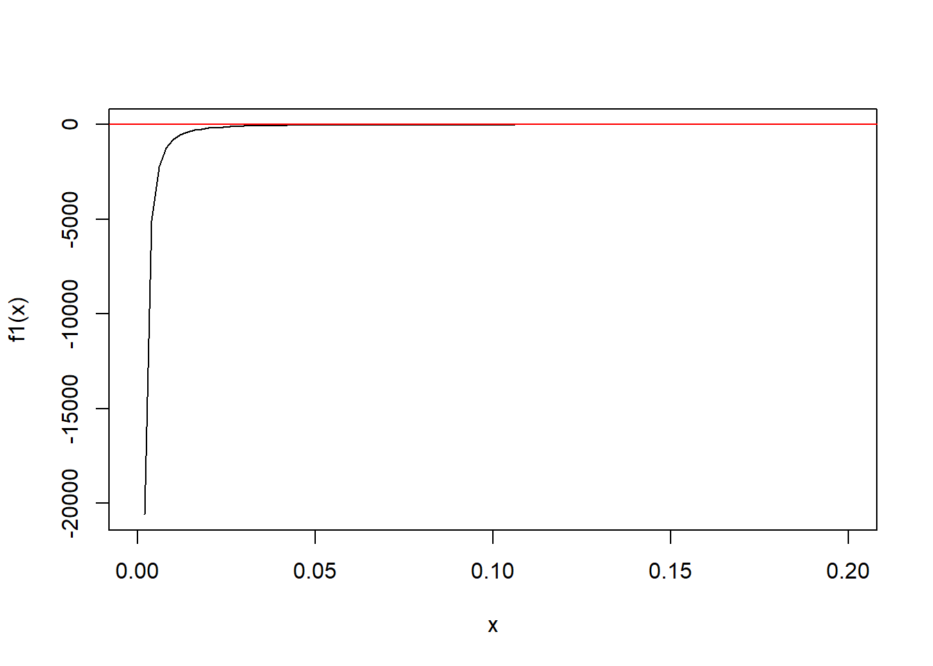
Figure 4.1: The difference between two constraints

We follow the author’s choice here, then the LHS of (4.9) is less than the following, \[\begin{equation} \frac{\left(1+\rho_{w}^{2}\right) \rho_{w}^{2}}{\left(1-\rho_{w}^{2}\right)}\alpha^{2}\left[\frac{\left(2+6 \rho_{w}^{2}\right)}{\left(1-\rho_{w}^{2}\right)}\|\mathbf{W}-\mathbf{I}\|^{2} L^{2}+\frac{\left(1-\rho_{w}^{2}\right)}{4 \rho_{w}^{2}} L^{2}\right]\leq RHS=\frac{\left(1-\rho_{w}^{2}\right)^{2}}{4 \Gamma} \tag{4.13} \end{equation}\] Hence, it suffice to make \(\alpha\), \[\begin{equation} \alpha\leq \frac{\left(1-\rho_{w}^{2}\right)^{2}}{2 \sqrt{\Gamma} L \max \left(6 \rho_{w}\|\mathbf{W}-\mathbf{I}\|, 1-\rho_{w}^{2}\right)}\leq \frac{\left(1-\rho_{w}^{2}\right)^{2}}{L \sqrt{\Gamma\left(1+\rho_{w}^{2}\right)} \sqrt{4 \rho_{w}^{2}\left(2+6 \rho_{w}^{2}\right)\|\mathbf{W}-\mathbf{I}\|^{2}+\left(1-\rho_{w}^{2}\right)^{2}}} \end{equation}\]

The latter inequality comes from \(\rho_w^2<1<\frac{7}{6}\) and \(a+b\leq 2\max(a,b)\).

For the inequality (4.10), from the inequality (4.9), it is sufficient to have \[\begin{equation} a_{12} a_{23} a_{31}\leq \frac{(\Gamma-1)}{\Gamma(\Gamma+1)}\left(1-a_{11}\right)\left(1-a_{22}\right)\left(1-a_{33}\right) \end{equation}\]

Thus,

\[\begin{equation} \alpha \leq \frac{\left(1-\rho_{w}^{2}\right)}{3 \rho_{w}^{2 / 3} L}\left[\frac{\mu^{2}}{L^{2}} \frac{(\Gamma-1)}{\Gamma(\Gamma+1)}\right]^{1 / 3} \end{equation}\] Then, when the step size \(\alpha\) is chosen such that \[\begin{equation} \alpha \leq \min \left\{\frac{\left(1-\rho_{w}^{2}\right)}{12 \rho_{w} L}, \frac{\left(1-\rho_{w}^{2}\right)^{2}}{2 \sqrt{\Gamma} L \max \left\{6 \rho_{w}\|\mathbf{W}-\mathbf{I}\|, 1-\rho_{w}^{2}\right\}}, \frac{\left(1-\rho_{w}^{2}\right)}{3 \rho_{w}^{2 / 3} L}\left[\frac{\mu^{2}}{L^{2}} \frac{(\Gamma-1)}{\Gamma(\Gamma+1)}\right]^{1 / 3}\right\} \tag{4.14} \end{equation}\]

we have \(\rho(A_{dsgt})<1\).